A key concept in statistics is variability. This concept is really nothing more than the idea that individual objects or events differ from one another. For instance, the monthly cost of personal transportation (car, bus, biking, etc.) obvious varies from one person to another; some people spend a lot on transportation, some very little.
Common sense says that some of the variability can be explained or accounted for by factors that can themselves be measured. For instance, the monthly cost of transportation depends on a person’s commuting distance to work, on the availability and practicality of using public transportation such as a bus or low-cost transportation such as a bicycle. These factors that can account for the variability are called explanatory variables. The quantity whose variability we want to account for with the explanatory variables is called the response variable.
This workbook is about the process of accounting for the variation in a response variable, how to say meaningfully “how much” of that variation the explanatory variables account for, how much a change in an explanatory variable will lead to a change in the response variable, and even whether a proposed explanatory variable (say whether or not a car has fuzzy dice on the dashboard) can be shown to account for the variability or not. (Fuzzy dice? We think not. But how would you convince a fuzzy-dice fan?)
The goal of statistical analysis of data is to give answers – supported by data! – to questions like these:
- Does a given explanatory variable account for the response variable at all?
- If it does, how strong is the explanatory variable in accounting for variation?
To answer these questions, you need to have data, and the process of collecting data is itself a matter worth going into in detail. This workshop starts at the point where you already have data, you have decided what the response variable is going to be (for instance, the monthly cost of transportation), and you have ideas for what explanatory variables you want to know (for instance, distance to work, car or bus, and so on).
Once you are at this point, you’re ready to start the steps demonstrated in this workbook. These are:
- Measure the amount of variability in the response variable.
- Build a function that takes the explanatory factors and inputs and returns as output a best guess for the response variable.
- Measure the amount of variability in the best guesses from the function.
- Translate the measurements from (1) and (3) into a form that addresses the particular question(s) you have in mind.
Measure the amount of variability in the response variable
The response variable in your data will usually have one of the two most common forms for data:
The response variable is a number and so your data look like a set of numbers. For instance, if the response variable were the temperature outdoors, it might look like:
54, 61, 65, 58, 55, 45, 51, …
The response variable is a category describing some event, say whether it rained or not on each day. So, it might look like this:
rain, none, none, rain, rain, rain, none, …
As it happens, you’ll measure the variability in both kinds of variables – numerical or categorical – in much the same way. But there is an extra step for categorical variables. You need first to translate each category into a number, say 1 for rain and 0 for no rain.
ACTIVITY: Translate a categorical variable into zeros and ones.
IDEA:
- Graphics for calculating the amount of variability.
- Arithmetic for calculating the amount of variability. \(2 \sqrt{p(1-p)}\)
Res <- list()
n <- 1000
phat <- seq(.1, .9, by = 0.1)
for (k in seq_along(phat)) {
  Res[[k]] <- data.frame(y = sample(0:1, size = n, replace = TRUE,
                                  prob = c(phat[k], 1 - phat[k])),
                         prop = phat[k])
}
Res <- dplyr::bind_rows(Res)
Stats <- data.frame(p = phat, spread = sqrt(phat*(1-phat)))
gf_jitter(y ~ prop, data = Res, alpha = 0.1, height = 0.1) %>%
  gf_errorbar(spread + spread ~ phat, data = Stats)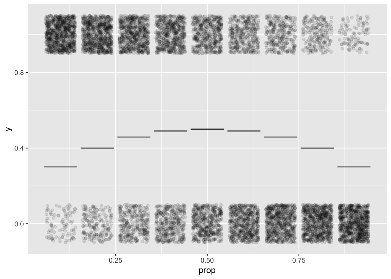
D <- data.frame(y = sample(c(0,0,1), replace = TRUE, size = 500))
gf_jitter(y ~ 1, data = D, height = 0.1) %>%
  gf_lims(x = c(0,2))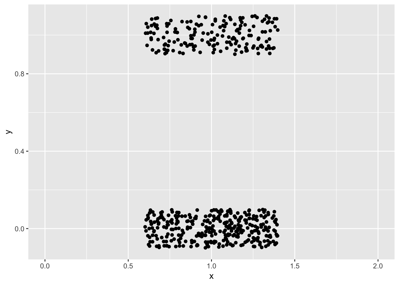
Step 1. Find the summary interval of the variable.
Step 3. Measure the length of the summary interval giving your result: how much variability there is